In my last post, I wrote about two infinite games whose analysis leads to interesting questions about subsets of the real numbers. In this post, I will talk about two more infinite games, one related to the Baire Category Theorem and one to Diophantine approximation. I’ll then talk about the role which such Diophantine approximation questions play in the theory of dynamical systems.
The Choquet game and the Baire Category Theorem
The Cantor game from Part I of this post can be used to prove that every perfect subset of  is uncountable. There is a similar game which can be used to prove the Baire Category Theorem. Let
  be a metric space. In Choquet’s game, Alice moves first by choosing a non-empty open set
  in . Then Bob moves by choosing a non-empty open set
  . Alice then chooses a non-empty open set
  , and so on, yielding two decreasing sequences
  and
and  of non-empty open sets with
  for all
  . Note that
  ; we denote this set by
  . Alice wins if is empty, and Bob wins if is non-empty.
Exercise 1: Show that if is complete (i.e., every Cauchy sequence converges) then Bob has a winning strategy. [Hint: If  is a decreasing sequence of closed sets in whose diameter tends to zero then
  .]
.]
Exercise 2: Show that if contains a non-empty open set  which is meager (i.e., is a countable union of closed sets with empty interior), then Alice has a winning strategy. [Hint: Alice starts with
  and responds to each choice of Bob’s with
  .]
.]
Combining these two observations, we obtain the Baire Category Theorem:
A non-empty complete metric space cannot be meager.
The Baire Category Theorem is used in functional analysis to prove the Open Mapping Theorem, Closed Graph Theorem, and Uniform Boundedness Principle. See this page for some other interesting applications (my personal favorite being the fact that the field  is not complete). The Baire Category Theorem will make a guest appearance below in our discussion of Cremer points for complex dynamical systems.
Diophantine numbers
An irrational number  is said to be Diophantine (of order at most
  ) if there exists
  so that
  for every rational number
  . By a theorem of Liouville, an algebraic number of degree
  is Diophantine of order at most . Non-Diophantine irrational numbers, which are therefore transcendental, are often called Liouville numbers. The first proof of the existence of transcendental numbers, by Liouville in 1844, combined the above theorem with the observation that well-approximated numbers such as
  are non-Diophantine. (Cantor later gave a simple non-constructive proof of the existence of transcendental numbers using his theorem that is uncountable.) While Liouville numbers are dense in the real line, they are rare in the sense that the Hausdorff dimension of the set of all Liouville numbers is zero.
By a famous 1955 theorem of Klaus Roth (for which he won a Fields Medal), every algebraic irrational number is Diophantine of order  for every . This result and its subsequent generalizations (such as Schmidt’s Subspace Theorem) are incredibly important in the modern subject of Diophantine Geometry; see for example this survey paper by Corvaja and Zannier.
Schmidt’s Game and Badly Approximable Numbers
It is an exercise using the pigeonhole principle to see that there are no Diophantine numbers of order less than 2. Diophantine numbers of order exactly 2 are called badly approximable; another name for them is bounded type, since being Diophantine of order 2 is equivalent to having bounded continued fraction coefficients. These are the ‘most Diophantine’ numbers. Although the set of badly approximable numbers is small in the sense that it has Lebesgue measure zero, it is also rather large in the sense that it has Hausdorff dimension 1. The latter fact was proved by Wolfgang Schmidt via an infinite two-player game played on the real number line.
Schmidt’s game goes as follows. Fix real numbers  and a subset
  of the real line. First Bob picks a closed interval
  . Then Alice picks a closed interval
  whose length is
  times the length of . Next Bob chooses a closed interval
  whose length is
  times the length of
  . Alice then picks a closed interval
  whose length is times the length of
  , and so on. Alice wins the game if
  , and Bob wins the game if
  .
.
Winning sets
We say that is a winning set if there exists an  such that Alice has a winning strategy for all
  . Schmidt proved that the set of badly approximable numbers has Hausdorff dimension 1 by establishing the following two facts:
- Every winning set has Hausdorff dimension 1.
- The set of all badly approximable real numbers is winning.
Schmidt also describes various other winning sets, e.g. the set of real numbers with infinitely many zeros in their base 10 representation.
Interlude: Complex dynamical systems
Much of the theory of dynamical systems centers around the problem of determining whether a periodic orbit is stable or unstable. Such questions originally arose in celestial mechanics, and are known to be extremely difficult. There is a model of this situation in complex dynamics which is much simpler than the case of planetary motion, yet still rich enough to hold subtle and interesting surprises.
In the theory of dynamics of one complex variable, as pioneered by Fatou and Julia, one starts with a rational function  of degree at least 2 and studies the behavior of points of
  under iteration. The “stable” locus, consisting of points whose nearby neighbors stay close together under iteration, is called the Fatou set. (More precisely, the Fatou set consists of all points with an open neighborhood on which the iterates of
  form an equicontinuous family.) Its complement, the Julia set, consists of the “unstable” points for which the orbits of even very small neighborhoods eventually get very big. (For a wealth of information about Fatou and Julia sets, the reader should consult Milnor’s excellent book “Dynamics in One Complex Variable”.) One of the key problems in the theory is to determine under what conditions a periodic point belongs to the Fatou set (resp. Julia set).
For this, one associates to every periodic point a complex number  called its multiplier. (For a fixed point, the multiplier is just the derivative of ; for the general case see for example this blog post of mine.) If
  , the periodic point is called repelling and belongs to the Julia set. If
  , the periodic point is called attracting and belongs to the Fatou set. These results are easy, but the case where
  (where the periodic point is called indifferent) is much more delicate. In this case, write
  with
with  ; the number is called the rotation number. If is a root of unity, i.e., is rational, then the periodic point belongs to the Julia set. (This is also an easy result, though understanding what iteration near such a point looks like can be quite subtle.) Much harder to understand is the case where is not a root of unity, i.e., is irrational; such a periodic point is called irrationally indifferent. In this case, whether the periodic point belongs to the Fatou set or the Julia set turns out to depend on how well can be approximated by rational numbers.
Let us assume for simplicity that the periodic point in question is a fixed point at the origin, so that  near the origin. The key lemma in this situation is that an indifferent fixed point lies in the Fatou set if and only if is locally linearizable, meaning that there is a local holomorphic change of coordinates
  which conjugates to the rotation
  , i.e.,
  in a neighborhood of the origin. In 1927, Hubert Cremer proved that for a generic choice of , a rational function of degree at least 2 having the origin as an (irrationally) indifferent fixed point of rotation number is not locally linearizable, hence the origin belongs to the Julia set. Here generic means that it holds for a set
  containing a countable intersection of dense open subsets of
  ; by the Baire Category Theorem, such a set must be dense and uncountable.
Diophantine approximation and Siegel discs

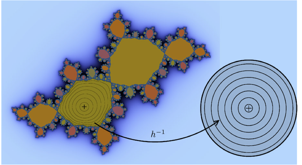
A Siegel disc.
It was an open problem whether Cremer’s theorem could be extended to all until Carl Ludwig Siegel proved in 1942 that if the irrational number is Diophantine then is locally linearizable, hence the origin belongs to the Fatou set. The corresponding component of the Fatou set, on which is conformally conjugate to an irrational rotation of the unit disc, is called a Siegel disc. Siegel’s proof of the existence of such irrational rotation domains, and the appearance of Diophantine approximation in this context, was a major milestone in the theory of dynamical systems.
The set of Diophantine numbers is dense in and has full Lebesgue measure and Hausdorff dimension one. This means that, for a different but perfectly reasonable meaning of the word generic, Cremer’s theorem is completely wrong! As we saw from Schmidt’s game, the very special Diophantine numbers of bounded type already have Hausdorff dimension one.
Concluding remarks
1. For much more on infinite games played on the real number line, including a detailed history of the subject, see Telgarsky’s survey paper Topological games: On the 50th anniversary of the Banach-Mazur game. See also this Wikipedia page. My exposition of Choquet’s game is based on an exercise in the book Elements of Functional Analysis by Hirsch and Lacombe (Springer Graduate Texts in Mathematics 192, 1999).
2. Quadratic irrationals are badly approximable; it is unknown whether there are any other algebraic numbers which are badly approximable.
3. Some interesting variants of Schmidt’s Game are discussed in Curt McMullen’s paper Winning sets, quasiconformal maps, and Diophantine approximation. My exposition of Schmidt’s Game was influenced by the discussion in that paper.
4. For an excellent elementary introduction to the role of Diophantine conditions in the theory of dynamical systems, I recommend this article by Fields Medalist Jean-Christophe Yoccoz in the compilation “An Invitation to Mathematics” by Schleicher and Lackmann. (Our picture of a Siegel disc was taken from that article.) In particular, the reader can learn there about Brjuno numbers, which are more general than Diophantine numbers and also imply local linearlizability. Yoccoz proved in 1987 that if is a quadratic polynomial with irrational rotation number at the origin, then it is locally linearizable if and only if is a Brjuno number. It is unknown whether local linearizability implies that is Brjuno for more general rational (or even polynomial) maps .
5. Diophantine conditions on rotation numbers come up in the study of all sorts of dynamical systems, not just complex dynamics. For example, Herman and Yoccoz proved that if is a real-analytic diffeomorphism of whose rotation number  is Diophantine, then is real-analytically conjugate to the rotation
 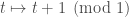 . If is
  , they also proved the converse to this statement. Diophantine conditions also show up in celestial mechanics and related dynamical systems, in the context of the vast subject now known as KAM theory.
6. Although quite different in flavor from the games we’ve been considering in this post (since it involves a finite game), I can’t help mentioning this award-winning paper by David Gale which uses the fact that at least one player always wins the game of Hex to give a simple proof of the Brouwer Fixed Point Theorem in topology. In fact, Gale establishes the equivalence of these two results! There is also an exposition of Gale’s results in this blog post. In this post, it is shown that the Brouwer Fixed Point Theorem implies a version of the Jordan Curve Theorem which in turn implies that there is always exactly one winner in Hex.
7. If you know other examples of games which can be used to prove interesting mathematical theorems, please post to the comments section below!

Pingback: Real Numbers and Infinite Games, Part I | Matt Baker's Math Blog
Respectfully, there may be an error in the statement of the Baire Category Theorem. For example, \{0,1,2 \} is a non-empty subset of a complete metric space, but is certainly meager.
Thank you, I had left out the word “open”. But in any case the usual formulation of the BCT is just that X itself cannot be meager (if it’s a non-empty complete metric space), so I’ve changed the statement to this.
Excuse me, I am a student from Taiwan and wish to use the figure in this post to explain the concept of Siegel disk. I want to know if it is okay to put in on my poster. Thank you.
Sure, though I myself got it from somewhere else. (I wish I remembered from where, I should have documented that…)