Lorentzian polynomials I: Theory

I’m organizing a reading seminar this semester on Lorentzian polynomials, mainly following this paper by Brändén and Huh but also covering some of the work of Anari et. al. In this post, I’d like to give a quick introduction to this active and beautiful subject. I’ll concentrate on the basic theory for now, and in a follow-up post I’ll discuss some of the striking applications of this theory.

One major goal of the theory of Lorentzian polynomials is to provide new techniques for proving that various naturally-occurring sequences of non-negative real numbers $a_k$ are log-concave, meaning that $a_k^2 \geq a_{k-1} a_{k+1}$ for all $k$ . More generally, the authors consider homogeneous multivariate polynomials $p(x_1,\ldots,x_n)$ with non-negative coefficients and study certain natural extensions of log-concavity to this setting. (For some background on log-concave sequences, see this survey paper which I wrote for the Bulletin of the AMS.) So let me begin by introducing two “classical” methods for proving (an even sharper version of) log-concavity of the coefficients of certain polynomials.

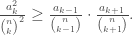
Method #1 (Newton): Let $p(x) = \sum_{k=0}^n a_k x^k$ be real-rooted univariate polynomial with non-negative coefficients. Then the sequence of coefficients of $p(x)$ is ultra-log-concave (ULC), meaning that $\frac{a_k^2}{\binom{n}{k}^2} \geq \frac{a_{k-1}}{\binom{n}{k-1}} \cdot \frac{a_{k+1}}{\binom{n}{k+1}}.$

Note that ultra-log-concavity is stronger than log-concavity (simple exercise).

Slick proof of Newton’s theorem: The idea is to reduce to the case of quadratic polynomials, where the result follows immediately from the fact that the discriminant of a real-rooted quadratic must be non-negative, using the following two operations which preserve real-rootedness:

(1) Differentiation: If $p(x)$ is real-rooted, then by Rolle’s theorem so is $p'(x)$ . (In fact, the roots of $p'(x)$ interlace the roots of $p(x)$ , but we won’t explicitly need this fact.)

(2) Reciprocation: If $p(x) = \sum_{k=0}^n a_k x^k$ is real-rooted, then so is the reciprocal polynomial $r(x) = \sum_{k=0}^n a_{n-k} x^k.$ (This is clear once you realize that $r(x) = x^n p(1/x).$ )

The proof is now easy: fix $1 \leq k \leq n-1$ and differentiate $p(x)$ $k-1$ times in order to get rid of all the coefficients $a_i$ with $i < k-1$ . Now form the reciprocal polynomial of $p^{k-1}(x)$ and differentiate it $n-k-1$ times in order to get rid of all the coefficients $a_i$ with $i > k+1$ . What remains is the real-rooted quadratic polynomial $q(x) = \frac{(k-1)!(n-k-1)!}{2} a_{k-1}x^2 + k!(n-k)! a_k x + \frac{(k+1)!(n-k-1)!}{2} a_{k+1}.$ Applying the inequality ${\rm Disc}(q) \geq 0$ and doing some routine algebra gives the desired ultra-log-concavity. Q.E.D.

A couple of quick observations about this argument:

(1) The “routine algebra” at the end, as well as the apparent cleverness required to think of the reciprocation trick, disappears if we instead consider homogeneous polynomials of the form $f(x,y) = \sum_{k=0}^n \frac{c_k}{k! (n-k)!} x^k y^{n-k}.$ If we assume that $f(x,1)$ (or, equivalently, $f(1,y)$ ) is real-rooted, then differentiating $k-1$ times with respect to $x$ and $n-k-1$ times with respect to $y$ gives a cleaner-looking homogeneous quadratic polynomial whose discriminant must be non-negative, yielding immediately (with no extra algebraic manipulations) log-concavity of the sequence $c_k$ , which is easily seen to be equivalent to ultra-log-concavity of the sequence $a_k = \frac{c_k}{k! (n-k)!}.$ For this reason and others, we will always work in what follows with homogenous polynomials written in “exponential generating function” form.

(2) The argument does not actually require that $f(x,1)$ be real-rooted, just that after any suitable sequence of partial differentiations we end up with a real-rooted quadratic. This observation will help motivate the definition of Lorentzian polynomials below.

Method #2 (Cauchy, Sylvester): Suppose $f(x,y)= \frac{1}{2} \sum_{i=1}^n c_{ii} x_i^2 + \sum_{i\neq j} c_{ij} x^i y^j$ is a symmetric quadratic form with $c_{ii} > 0$ for all $i$ and having Lorentzian signature $(1,n-1)$ (i.e., the symmetric matrix $C = (c_{ij})$ has one positive and $n-1$ negative eigenvalues). Then every minor of $C$ has Lorentzian signature as well, and in particular we have $c_{ij}^2 > c_{ii} c_{jj}$ for all $i,j$ .

Proof: By Cauchy’s interlacing theorem, the eigenvalues of every principal minor $\hat{C}_i$ of $C$ interlace the eigenvalues of $C$ . In particular, $\hat{C}_i$ must have signature either $(0,n-1)$ or $(1,n-2)$ . However, the former is impossible since the trace of $C$ and $\hat{C}_i$ are both positive. By induction, it follows that every minor of $C$ has Lorentzian signature. Applying this to the $2\times 2$ minor $C_{ij}$ of $C$ corresponding to rows $i$ and $j$ , it follows that ${\rm det}(C_{ij}) < 0$ , hence the stated inequality. Q.E.D.

Note that in both the Newton and Cauchy-Sylvester methods, log-concavity is ultimately proved by reducing to the case of homogeneous polynomials of degree 2. We will describe a general class of homogenous polynomials for which one can reduce log-concavity considerations to the case of Lorentzian quadratic forms via partial differentiation. In order to do this, we must first fix some notation.

(1) Let $H^d_n = \sum_{\alpha \in \Delta^d_n} \frac{c_\alpha}{\alpha!} x^\alpha$ be the set of homogenous polynomial of degree $d$ in $n$ variables $x_1,\ldots,x_n$ , where $\Delta^d_n = \{ \alpha = (\alpha_1,\ldots,\alpha_n) \in {\mathbb N}^n \; : \; \sum_k \alpha_k = d \},$ $x^\alpha = x_1^{\alpha_1} \cdots x_n^{\alpha_n}$ , and $\alpha! = \alpha_1 ! \cdots \alpha_n!$ . (We assume throughout this post that $d \geq 2$ .)

(2) Let $P^d_n$ be the set of all $f \in H^d_n$ having positive coefficients, and let $\mathring{L}^2_n$ be the set of all homogeneous quadratic forms $f \in P^2_n$ such that the Hessian matrix $H_f = ( \partial^i \partial^j f )$ has Lorentzian signature.

(3) For $d > 2$ , let $\mathring{L}^d_n$ be the set of all $f \in P^d_n$ such that $\partial^\alpha f \in \mathring{L}^2_n$ for all $\alpha \in \Delta^{d-2}_n$ . We call such polynomials strictly Lorentzian.

(4) Let $L^d_n$ be the closure of $\mathring{L}^d_n$ in the finite-dimensional vector space $H^d_n$ . We call $L^d_n$ the set of Lorentzian polynomials. Note that the coefficients of a Lorentzian polynomial must all be non-negative.

Although it’s not obvious, it turns out (and should at least seem plausible at this point) that the coefficients of a Lorentzian polynomial have the following generalized ultra-log-concavity property:

Theorem (Brändén-Huh): If $f = \sum_{\alpha \in \Delta^d_n} \frac{c_\alpha}{\alpha!} x^\alpha$ is Lorentzian, then $c_\alpha^2 \geq c_{\alpha + e_i - e_j} c_{\alpha - e_i + e_j}$ for all $i,j$ , where $e_i$ is the $i^{\rm th}$ standard basis vector in ${\mathbb Z}^n$ .

In addition, being Lorentzian implies a strong log-concavity property for the values of the polynomial:

Theorem (Brändén-Huh): If $f$ is Lorentzian, then $\log f$ is a concave function on the positive orthant ${\mathbb R}^n_{>0}.$ In fact, a homogeneous polynomial $f \in H^d_n$ with non-negative coefficients is Lorentzian if and only if $\log \partial^\alpha f$ is a concave function on ${\mathbb R}^n_{>0}$ for all $\alpha \in \Delta^{d-2}_n.$

In particular, if we can verify that a given homogeneous polynomial $f$ is Lorentzian, we obtain a whole suite of interesting inequalities satisfied by not only the coefficients of $f$ but also the values of $\log f$ . Because of the closure operation, however, it is not obvious from the definition how to check whether a polynomial is Lorentzian. We will turn to this issue next, after presenting a few examples and non-examples of Lorentzian polynomials. (Note: some of the following assertions are easy to check and others are much harder, but all are explained in the paper of Brändén-Huh.)

Example #1: ( $n=2$ ) A bivariate homogenous polynomial of degree $d$ with non-negative coefficients is Lorentzian if and only if the coefficients form an ULC sequence, i.e., they satisfy Newton’s inequalities. Note that this is more general than being real-rooted: for example, $f(x,y) = 2x^3 + 12x^2 y + 18x y^2 + 9y^3$ is Lorentzian but not real-rooted.

Example #2 ( $d=2$ ): A homogeneous quadratic form $f$ in $n$ variables with non-negative coefficients is Lorentzian if and only if the Hessian of $f$ has at most one positive eigenvalue.

Example #3: (A warning) For $d>2$ , being Lorentzian is not the same thing as checking that all partial derivatives of order $d-2$ are Lorentzian quadratic forms. (In other words, the closure operation does not “commute” with taking partial derivatives.) For example, one can show (see below) that $f(x,y)=x^3 + y^3$ is not Lorentzian despite the fact that both $\partial_x f$ and $\partial_y f$ are.

Example #4: A homogenous polynomial $f \in H^d_n$ with non-negative coefficients is called stable if $f(\ell(x))$ is real-rooted for all affine-linear maps $\ell : {\mathbb R} \to {\mathbb R}^n$ with positive gradient (i.e., $\ell(x) = ux + v$ with $u \in {\mathbb R}^n_{>0}$ and $v \in {\mathbb R}^n$ ). It turns out that a homogeneous stable polynomial is automatically Lorentzian. It was known prior to the work of Brändén-Huh et. al. that the coefficients of a stable polynomial are log-concave, so the new work can be viewed as a far-reaching generalization of this fact.

Example #5: If $P_1,\ldots,P_n$ are convex subsets of some Euclidean space ${\mathbb R}^N$ , the function ${\mathbb R}^n \to {\mathbb R}$ given by $f(w_1,\ldots,w_n) = {\rm Vol}(w_1 P_1 + \cdots + w_n P_n)$ (where addition denotes Minkowski sum) is a Lorentzian polynomial.

Example #6: The product of two Lorentzian polynomials is again Lorentzian.

In my follow-up post, I will give a several more non-trivial examples. But to conclude the present post, I’d like to focus on the important question of how to easily determine whether a polynomial $f \in H^d_n$ with non-negative coefficients actually belongs to $L^d_n$ or not.

It turns out that there is a purely combinatorial condition on the support of $f$ (i.e., the set of $\alpha \in \Delta^d_n$ such that $c_\alpha \neq 0$ ) which guarantees that taking closures in $H^d_n$ does, in a suitable sense, commute with taking partial derivatives. Somewhat miraculously, the combinatorial condition turns out to be intimately related to the notion of a matroid. (The reason this is so remarkable is that the definition we’ve given for Lorentizan polynomials would seem to have nothing whatsoever to do with matroids, it involves just basic linear algebra and multivariable calculus.)

More precisely, a subset $J \subset {\mathbb N}^n$ is called M-convex (or, equivalently, $J$ is the set of bases of a polymatroid) if for every $\alpha, \beta \in J$ and every index $i$ such that $\alpha_i > \beta_i$ , there exists an index $j$ with $\alpha_j < \beta_j$ such that $\alpha - e_i + e_j$ and $\beta - e_j + e_i$ both belong to $J$ .

Theorem (Brändén-Huh): The support of any Lorentzian polynomial is M-convex, and conversely every M-convex set is the support of a non-empty collection of Lorentzian polynomials.

A few remarks:

(1) If $J \subset \{ 0,1 \}^n$ , then $J$ is M-convex if and only if $J$ is the set of bases of a matroid. Thus M-convex sets are to matroids as multisets are to sets.

(2) From the theorem, we can see immediately why the polynomial $x^3 + y^3$ from Example #3 above is not Lorentzian: its support is “missing” the monomials $x^2 y$ and $y^2 x$ needed for M-convexity.

(3) An earlier theorem of Brändén asserts that the Fano matroid is not the support of any stable polynomial. So the intimate relationship between M-convexity and Lorentzian polynomials is only a one-way implication if we replace “Lorentzian” by “stable”.

Because there is no Euclidean closure in the statement, the following theorem leads to a straightforward algorithm for determining whether or not a given polynomial is Lorentzian:

Theorem (Brändén-Huh): Let $M^d_n$ be the set of all homogeneous polynomials $f \in H^d_n$ whose support is M-convex. Then $L^d_n = \{ f \in M^d_n \; : \; \partial^\alpha f \in L^2_n \; \forall \; \alpha \in \Delta^{d-2}_n \},$ where $L^2_n$ is the set of all $f \in H^2_n$ with non-negative coefficients whose Hessian has at most one positive eigenvalue (see Example #2 above).

Concluding remarks:

The notion of Lorentzian polynomial was independently discovered by Anari, Oveis Garan, and Vinzant at the same time as Brändén-Huh. Some of the applications given in these authors’ papers are similar to those of Brändén-Huh and some are quite different. I will discuss some of these applications in my next post.
The notion of M-convexity is due to Kazuo Murota, see this survey paper for further context. M-convex subsets of ${\mathbb N}^n$ are “cryptomorphically” equivalent to discrete polymatroids, which can be defined as non-decreasing submodular functions from $\{ 0,1 \}^n \to {\mathbb N}.$
Somewhat paradoxically, it is often easier (when true) to prove that a given polynomial is Lorentzian than to directly establish the strictly weaker fact that the polynomial is log-concave on the positive orthant. This type of “paradox”, where to prove a given statement it is often useful to prove something stronger, is rather ubiquitous in mathematics.
Thanks to Paolo Aluffi for pointing out an error in an earlier version of this post.

Matt Baker's Math Blog

Thoughts on number theory, graphs, dynamical systems, tropical geometry, pedagogy, puzzles, and the p-adics

Lorentzian polynomials I: Theory

4 thoughts on “Lorentzian polynomials I: Theory”

Leave a Reply Cancel reply

Share this:

Like this:

Related

4 thoughts on “Lorentzian polynomials I: Theory”

Leave a Reply Cancel reply