Pi and the AGM

In celebration of Pi Day 2024, I would like to explain how the “Arithmetic-Geometric Mean” of Gauss and Legendre can be used to give a rapid method for computing the digits of $\pi$ . By “rapid” here, I mean that the algorithm exhibits quadratic convergence: the number of correct digits roughly doubles with each iteration. I will mainly follow the exposition in Donald J. Newman’s 1985 paper “A Simplified Version of the Fast Algorithms of Brent and Salamin”.

The Arithmetic-Geometric Mean

Given positive real numbers $a$ and $b$ , define their arithmetic mean to be $A(a,b) := \frac{a+b}{2}$ and their geometric mean to be $G(a,b) = \sqrt{ab}$ . The Arithmetic-Geometric Mean, or AGM, of $a$ and $b$ is defined as $M(a,b) := \lim_{n \to \infty} a_n = \lim_{n \to \infty} b_n$ , where $(a_0,b_0) = (a,b)$ and $(a_n,b_n) = (A(a_{n-1},b_{n-1}),G(a_{n-1},b_{n-1}))$ for $n \geq 1$ . In other words, if $T(a,b) = (A(a,b),G(a,b))$ , then $M(a,b) = \lim_{n \to \infty} T^{(n)}(a,b)$ , where $T^{(n)}$ denotes the $n^{\rm th}$ iterate of $T$ . It is not difficult to show that the number of digits in which $a_n$ and $b_n$ agree roughly doubles with each iteration of $T$ , i.e., the iteration scheme converges quadratically. Indeed, we have

$a_{n+1} - b_{n+1} = \frac{(\sqrt{a_n} - \sqrt{b_n})^2}{2} = \frac{(a_n - b_n)^2}{2(\sqrt{a_n} + \sqrt{b_n})^2} \leq \frac{1}{8b_1} (a_n - b_n)^2.$

For example, if $a = 24$ and $b = 6$ , then $(a_3,b_3) = (13.458203\ldots,13.458139\ldots)$ and $(a_4,b_4) = (13.458171481745\ldots,13.458171481706\ldots)$ . For comparison, we have $M(a,b) = 13.4581714817256\ldots$

The AGM first appeared in a paper of Lagrange, but it was Gauss who first connected it to the theory of elliptic integrals, which is the connection lying at the heart of the main formula in this post.

The Geometric-Harmonic Mean

Define the harmonic mean of $a$ and $b$ to be $H(a,b) := \frac{2ab}{a+b}$ . Rather than working with the AGM, it will actually be more convenient for us to work with the Geometric-Harmonic Mean, or GHM, of $a$ and $b$ , defined as $m(a,b) := \lim_{n \to \infty} a_n = \lim_{n \to \infty} b_n$ , where $(a_0,b_0) = (a,b)$ and $(a_n,b_n) = (G(a_{n-1},b_{n-1}),H(a_{n-1},b_{n-1}))$ .

Simple algebraic manipulations yield 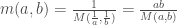$m(a,b) = \frac{1}{M(\frac{1}{a},\frac{1}{b})} = \frac{ab}{M(a,b)}$ . Note that since $m(ta,tb)= t\cdot m(a,b)$ , we have $m(a,b)=b \cdot m(\frac{a}{b},1)$ , so the single-variable function $m(x,1)$ determines the two-variable function $m(a,b)$ .

Asymptotic formula for $m(N,1)$

The main result of this post is the following asymptotic formula for the GHM:

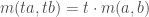
Theorem 1: $m(N,1) = \frac{2}{\pi} {\rm log}(4N) + O(\frac{1}{N^2})$ , where $\log$ denotes the natural logarithm.

From this formula, we can easily derive a rapidly converging algorithm for computing $\frac{2}{\pi}$ , and hence $\pi$ . Indeed, we have $m(N+1,1)-m(N,1) = \frac{2}{\pi} \log(1 + \frac{1}{N}) + O(\frac{1}{N^2})$ . By Taylor’s approximation, $\log(1+x) = x + O(\frac{1}{x^2})$ , and thus $N \cdot \left( m(N+1,1)-m(N,1) \right) = \frac{2}{\pi} + O(\frac{1}{N})$ . After about $2n$ iterations of the GHM, we can compute the left-hand side of this formula (with $N = 10^n$ ), and hence $\frac{2}{\pi}$ , with approximately $n$ digits of precision.

A brief history of computing $\pi$

According to Chapter 11 of the book “Pi and the AGM” by Jonathan and Peter Borwein, as of 1973 the record for computing digits of $\pi$ was one million decimal digits, using a Machin-like formula expressing $\pi$ as a linear combination of special values of the arctan function.

In 1983, Kanada, Yoshino, and Tamura used an AGM-based algorithm similar to Theorem 1 above to calculate the first 16,777,216 digits of $\pi$ , setting a new world record.

Nowadays, it is most common to use the Chudnovsky algorithm, which itself is based on formulas for $\pi$ discovered by Ramanujan. This algorithm was used to calculate the first 100 trillion digits of $\pi$ in March 2022. The Chudnovsky/Ramanujan formula for $\pi$ , while quite powerful, is significantly more complicated to prove than the AGM-based algorithm discussed in this post.

Gauss’s Formula for the AGM

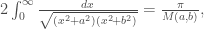
Our proof of Theorem 1 will use the following formula due to Gauss:

Theorem 2: $m(a,b) = \frac{2}{\pi} \int_{0}^\infty \frac{dx}{\sqrt{(1+\frac{x^2}{a^2})(1+\frac{x^2}{b^2})}}.$

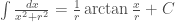
Proof: The integral 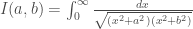$I(a,b) = \int_{0}^\infty \frac{dx}{\sqrt{(x^2+a^2)(x^2 + b^2)}}$ is invariant under $T$ ; indeed, the change of variables $t = \frac{1}{2} (x - \frac{ab}{x})$ gives (after some routine manipulation) $\int_{0}^\infty \frac{dx}{\sqrt{(x^2+a^2)(x^2 + b^2)}} = \int_{0}^\infty \frac{dt}{\sqrt{(t^2+((a+b)/2)^2)(t^2 + ab)}}.$ Applying this invariance repeatedly gives $2 \int_{0}^\infty \frac{dx}{\sqrt{(x^2+a^2)(x^2 + b^2)}} = \cdots = 2\int_{0}^\infty \frac{dx}{\sqrt{(x^2+M(a,b)^2)(x^2 + M(a,b)^2)}} = 2 \int_{0}^\infty \frac{dx}{x^2+M(a,b)^2}.$

The substitution $x = r \tan\theta$ shows that $\int \frac{dx}{x^2+r^2} = \frac{1}{r} \arctan \frac{x}{r} + C$ , and hence $2 \int_{0}^\infty \frac{dx}{\sqrt{(x^2+a^2)(x^2 + b^2)}} = \frac{\pi}{M(a,b)},$ which is equivalent to the stated formula. Q.E.D.

Proof of Theorem 1

By Theorem 2, we have 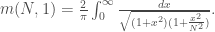$m(N,1) = \frac{2}{\pi} \int_{0}^\infty \frac{dx}{\sqrt{(1+x^2)(1+\frac{x^2}{N^2})}}.$ Since the substitution $x \mapsto \frac{N}{x}$ leaves the integrand invariant, we have $\int_0^{\sqrt{N}} L_N(x)dx = \int_{\sqrt{N}}^\infty L_N(x)dx$ , where $L_N(x) = \frac{1}{\sqrt{(1+x^2)(1+\frac{x^2}{N^2})}}$ . Thus $\int_{0}^\infty L_N(x)dx = \int_{0}^{\sqrt{N}} L_N(x)dx + \int_{\sqrt{N}}^\infty L_N(x)dx = 2 \int_{0}^{\sqrt{N}} L_N(x)dx.$

By the generalized binomial theorem, we have 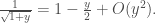$\frac{1}{\sqrt{1+y}} = 1 - \frac{y}{2} + O(y^2).$ Therefore $m(N,1) = \frac{4}{\pi} \int_{0}^{\sqrt{N}} L_N(x)dx = \frac{4}{\pi} \int_{0}^{\sqrt{N}} \frac{1}{\sqrt{(1+x^2)}} \left( 1 - \frac{x^2}{2N^2} + O(\frac{x^4}{N^4}) \right) dx.$

By the generalized binomial theorem once again, we have $\frac{x^2}{\sqrt{1+x^2}} = x \frac{1}{\sqrt{1 + \frac{1}{x^2}}} = x + O(\frac{1}{x}).$ Thus $m(N,1) = \frac{4}{\pi} \int_{0}^{\sqrt{N}} \frac{1}{\sqrt{(1+x^2)}} dx - \frac{4}{\pi} \int_{0}^{\sqrt{N}} \frac{x}{2N^2} dx+ O(\frac{1}{N^2}).$

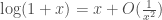
For $x \geq 0$ , the substitution $x = \tan \theta$ gives $\int \frac{1}{\sqrt{1+x^2}} dx = \log \left( x + \sqrt{1+x^2} \right) + C$ , and thus $m(N,1) = \frac{4}{\pi} \left( \log (\sqrt{N} + \sqrt{N+1}) - \frac{1}{4N} \right) + O(\frac{1}{N^2}).$

By Taylor’s theorem, $\log (\sqrt{N} + \sqrt{N+1}) = \log (2\sqrt{N}) + \frac{1}{4N} + O(\frac{1}{N^2}).$ Thus $m(N,1) = \frac{4}{\pi} \log (2\sqrt{N}) + O(\frac{1}{N^2}) = \frac{2}{\pi} \log (4N) + O(\frac{1}{N^2}).$ Q.E.D.

Concluding remarks

Gauss used Theorem 2 to prove that the arclength of the lemniscate $r^2 = \cos 2\theta$ is equal to $\frac{2\pi}{M(\sqrt{2},1)}$ . See David Cox’s paper “The Arithmetic-Geometric Mean of Gauss” for details, as well as a fascinating historical account of Gauss’s work on the subject.
From the introduction to Newman’s paper: “In their remarkable papers, Brent and Salamin, respectively, used the theory of elliptic functions to obtain “fast” computations of the function $e^x$ and of the number $\pi$ . In both cases rather heavy use of elliptic function theory, such as the transformation law of Landen, had to be utilized. Our purpose, in this note, is to give a highly simplified version of their constructions.”
A more “modern” application of the AGM is to the computation of periods. For example, if $E : y^2 = f(x)$ is an elliptic curve over ${\mathbb R}$ in Weierstrass form, with real roots $e_1 < e_2 < e_3$ , its period lattice is spanned by $\omega_1 = \frac{\pi}{M(\sqrt{e_3 - e_1},\sqrt{e_3-e_2})}$ and $\omega_2 = \frac{i\pi}{M(\sqrt{e_3 - e_1},\sqrt{e_2-e_1})}$ . This is, at least philosophically, related to Theorem 2 above.
Even though the complex square root is multi-valued, so it’s not clear a priori that the AGM of two complex numbers can even be defined, there is a satisfactory complex analogue of the AGM (due, as you might have guessed, to Gauss). Using the complex AGM, one can compute the period lattice of elliptic curves over ${\mathbb C}$ in a manner analogous to Remark 3 above.