John Forbes Nash and his wife Alicia  were tragically killed in a car crash on May 23, having just returned from a ceremony in Norway where John Nash received the prestigious Abel Prize in Mathematics (which, along with the Fields Medal, is the closest thing mathematics has to a Nobel Prize). Nash’s long struggle with mental illness, as well as his miraculous recovery, are depicted vividly in Sylvia Nasar’s book “A Beautiful Mind” and the Oscar-winning film which it inspired. In this post, I want to give a brief account of Nash’s work in game theory, for which he won the 1994 Nobel Prize in Economics. Before doing that, I should mention, however, that while this is undoubtedly Nash’s most influential work, he did many other things which from a purely mathematical point of view are much more technically difficult. Nash’s Abel Prize, for example (which he shared with Louis Nirenberg), was for his work in non-linear partial differential equations and its applications to geometric analysis, which most mathematicians consider to be Nash’s deepest contribution to mathematics. You can read about that work here.
On, now, to game theory. We will focus, for simplicity, on the theory of non-cooperative matrix games between two players 


For each 


Game theory began with the seminal 1928 paper of John von Neumann in which he proved the celebrated minimax theorem for zero-sum two-player games. Von Neumann defines a solution to the game to be a pair 


, and
.
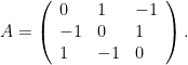
The remarkable and fundamental theorem proved by von Neumann is that every zero-sum two-player matrix game as above has a solution. To illustrate this with an example, suppose Player 1 and Player 2 each independently choose either rock, paper, or scissors, and the loser (according to the usual rules) pays the winner a dollar. This can be summarized by the payoff matrix
It is easy to check that 
For a more complicated example, suppose Player 1 is given the Ace of Diamonds, Ace of Clubs, and Two of Diamonds while Player 2 is given the Ace of Diamonds, Ace of Clubs, and Two of Clubs. Each player chooses one of his cards; Player 1 wins if the suits match and Player 2 wins if they do not. The amount of the payoff is the numerical value of the card chosen by the winner, with one exception: if both players choose their Two then the payoff is zero. This can be summarized by the payoff matrix

Exercise: Show that the mixed strategies 


An example of a non-zero sum game, to which von Neumann’s theorem does not apply but to which Nash’s theorem does, is the Prisoner’s Dilemma.
It is not difficult to show that von Neumann’s theorem is equivalent to the statement that for every zero-sum two-player matrix game, there exist mixed strategies 


We now turn to Nash’s extension of von Neumann’s fundamental theorem in which one does not assume the zero-sum condition. (Nash’s theorem also applies to any number of players, which represents another improvement over von Neumann, but for simplicity of exposition we will stick to the two-player scenario.) Nash discovered this result — and the key concept now known as “Nash equilibrium” — as a graduate student at Princeton in the summer of 1949. Nash told von Neumann’s secretary that he wanted to discuss an idea which might be of interest to the distinguished professor. As Sylvia Nasar writes:
Von Neumann was sitting at an enormous desk, looking more like a prosperous bank president than an academic in his expensive three-piece suit, silk tie, and jaunty pocket handkerchief. He had the preoccupied air of a busy executive. At the time, he was holding a dozen consultancies, “arguing the ear off Robert Oppenheimer” over the development of the H-bomb, and overseeing the construction and programming of two prototype computers. He gestured Nash to sit down. He knew who Nash was, of course, but seemed a bit puzzled by his visit.
He listened carefully, with his head cocked slightly to one side and his fingers tapping. Nash started to describe the proof he had in mind… But before he had gotten out more than a few disjointed sentences, von Neumann interrupted, jumped ahead to the as yet unstated conclusion of Nash’s argument, and said abruptly, “That’s trivial, you know. That’s just a fixed point theorem.”
…[Nash] never approached von Neumann again. Nash later rationalized von Neumann’s reaction as the naturally defensive posture of an established thinker to a younger rival’s idea, a view that may say more about what was in Nash’s mind when he approached von Neumann than about the older man. Nash was certainly conscious that he was implicitly challenging von Neumann. Nash noted in his Nobel autobiography that his ideas “deviated somewhat from the ‘line’ (as if of ‘political party lines’) of von Neumann and Morgenstern’s book”.
A few days after the disastrous meeting with von Neumann, Nash accosted [fellow graduate student] David Gale… Unlike von Neumann, Gale saw Nash’s point… Gale realized that Nash’s idea applied to a far broader class of real-world situations than von Neumann’s notion of zero-sum games. “He had a concept that generalized to disarmament”, Gale said later. But Gale was less entranced by the possible applications of Nash’s idea than its elegance and generality. “The mathematics was so beautiful. It was so right mathematically.”
Gale suggested asking a member of the National Academy of Sciences to submit the proof to the academy’s monthly proceedings. “He was spacey. He would never have thought of doing that,” Gale said recently, “so he gave me his proof and I drafted the NAS note.”… Gale added later, “I certainly knew right away that it was a thesis. I didn’t know it was a Nobel.”
To explain Nash’s theorem, we first need an extension of the setup used above. Suppose 


A Nash equilibrium is a pair 


With this terminology, Nash’s fundamental theorem is:
A Nash equilibrium exists for every (not necessarily zero-sum) matrix game.
Nash’s original proof of this theorem was based on the Kakutani fixed point theorem, a generalization of the more standard Brouwer fixed point theorem which was invented by Kukutani to streamline and clarify von Neumann’s complicated original proof of the minimax theorem. Nash later found an elegant argument based on the Brouwer fixed point theorem itself, which states that if 
Proof: Let 


We claim that 


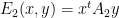
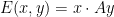
Now define a continuous map 

We claim that a pair of mixed strategies 


One direction of the claim is clear: if 


As a final coda to this post, we note that Brouwer fixed point theorem itself is equivalent to a certain theorem proved by John Nash about the game of Hex, which Nash himself invented as an undergraduate. (Hex was invented independently by a Danish man named Piet Hein, who marketed the game with Parker Brothers in the mid-1950’s.) A number of Nash’s fellow grad students recall thinking that Nash spent all of his time at Princeton in the common room playing board games. One morning in the winter of 1949, Nash ran into David Gale and shouted “Gale! I have an example of a game with perfect information. There’s no luck, just pure strategy. I can prove that the first player always wins, but I have no idea what his strategy will be. If the first player loses at this game, it’s because he’s made a mistake, but nobody knows what the perfect strategy is.”
The game board for Hex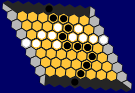 consists of a rhombus tiled by
When Gale finally understood what Nash was trying to tell him, he was captivated… The game quickly swept across the common room. It brought Nash many admirers, including the young John Milnor, who was beguiled by its ingenuity and beauty… Nash’s proof [that there can never be a draw, and thus that the first player can always win] is extremely deft, “marvelously non-constructive” in the words of [John] Milnor, who plays it very well. If the board is covered by black and white pieces, there’s always a chain that connects black to black or white to white, but never both. As Gale put it, “You can walk from Mexico to Canada or swim from California to New York, but you can’t do both.”
In his lovely paper “The Game of Hex and the Brouwer Fixed-Point Theorem”, David Gale writes:
The application of mathematics to games of strategy is now represented by a voluminous literature. Recently there has also been some work which goes in the other direction, using known facts about games to obtain mathematical results in other areas. The present paper is in this latter spirit. Our main purpose is to show that a classical result of topology, the celebrated Brouwer Fixed-Point Theorem, is an easy consequence of the fact that Hex, a game which is probably familiar to many mathematicians, cannot end in a draw. This fact is of some practical as well as theoretical interest, for it turns out that the two-player, two-dimensional game of Hex has a natural generalization to a game of n players and n dimensions, and the proof that this game must always have a winner leads to a simple algorithm for finding approximate fixed points of continuous mappings. This latter subject is one of considerable current interest, especially in the area of mathematical economics. This paper has therefore the dual purpose of, first, showing the equivalence of the Hex and Brouwer Theorems and, second, introducing the reader to the subject of fixed-point computations.
I should say that over the years I have heard it asserted in “cocktail conversation” that the Hex and Brouwer Theorems were equivalent, and my colleague John Stallings has shown me an argument which derives the Hex Theorem from familiar topological facts which are equivalent to the Brouwer Theorem. The proof going in the other direction only occurred to me recently, but in view of its simplicity it may well be that others have been aware of it. The generalization to n dimensions may, however, be new.
We encourage the reader to check out Gale’s article, as well as this blog post.
Concluding remarks:
1. Nash also made many other profound contributions to mathematics, including my own field of algebraic geometry; for example, he proved that given any smooth compact 


2. My exposition of von Neumann’s minimax theorem was heavily influenced by Harold W. Kuhn’s book “Lectures on the Theory of Games”.
3. One can prove Nash’s theorem on the game of Hex by elementary means; see for example this paper by Berman or this paper by Huneke. Combined with Gale’s theorem, these arguments give elementary proofs of the Brouwer Fixed-Point theorem. My exposition of the fact that the first player can always win in Hex was adopted from this AMS feature column.
4. For a mathematical analysis of the bar scene where Russell Crowe, as John Nash, explains his notion of equilibrium in the movie “A Beautiful Mind”, see this blog post.

Pingback: The Story of Nash Equilibrium: From Beautiful Mind to Beautiful Math - gametheorytimes.com