In this post I will provide a gentle introduction to the theory of martingales (also called “fair games”) by way of a beautiful proof, due to Johan Wästlund, that there are precisely labeled trees on vertices.

Apertif: a true story

In my early twenties, I appeared on the TV show Jeopardy! That’s not what this story is about, but it’s the reason I found myself in the Resorts Casino in Atlantic City, where the Jeopardy! tryouts were held (Merv Griffin owned both the TV show and the casino). At the time, I had a deep ambivalence (which I still feel) toward gambling: I enjoyed the thrill of betting, but also believed the world would be better off without casinos preying on the poor and vulnerable in our society. I didn’t want to give any money to the casino, but I did want to play a little blackjack, and I wanted to be able to tell my friends that I had won money in Atlantic City. So I hatched what seemed like a failsafe strategy: I would bet $1 at the blackjack table, and if I won I’d collect $1 and leave a winner. If I lost the dollar I had bet in the first round, I’d double my bet to $2 and if I won I’d stop playing and once again leave with a net profit of $1. If I lost, I’d double my bet once again and continue playing. Since I knew the game of blackjack reasonably well, my odds of winning any given hand were pretty close to 50% and my strategy seemed guaranteed to eventually result in walking home with a net profit of $1, which is all I wanted to accomplish. I figured that most people didn’t have the self-discipline to stick with such a strategy, but I was determined.

Here’s what happened: I lost the first hand and doubled my bet to $2. Then I lost again and doubled my bet to $4. Then I lost again. And again. And again. In fact, 7 times in a row, I lost. In my pursuit of a $1 payoff, I had just lost $127. And the problem was, I didn’t have $128 in my wallet to double my bet once again, and my ATM card had a daily limit which I had already just about reached. And frankly, I was unnerved by the extreme unlikeliness of what had just happened. So I tucked my tail between my legs and sheepishly left the casino with a big loss and nothing to show for it except this story. You’re welcome, Merv.

Martingales

Unbeknownst to me, the doubling strategy I employed (which I thought at the time was my own clever invention) has a long history. It has been known for hundreds of years as the “martingale” strategy; it is mentioned, for example, in Giacomo Casanova‘s memoirs, published in 1754 (“I went [to the casino of Venice], taking all the gold I could get, and by means of what in gambling is called the martingale I won three or four times a day during the rest of the carnival.”) Clearly not everyone was as lucky as Casanova, however (in more ways than one). In his 1849 “Mille et un fantômes”, Alexandre Dumas writes, “An old man, who had spent his life looking for a winning formula (martingale), spent the last days of his life putting it into practice, and his last pennies to see it fail. The martingale is as elusive as the soul.” And in his 1853 book “Newcomes: Memoirs of a Most Respectable Family”, William Makepeace Thackeray writes, “You have not played as yet? Do not do so; above all avoid a martingale if you do.” (For the still somewhat murky origins of the word ‘martingale’, see this paper by Roger Mansuy.)

The mathematical theory of martingales was initiated by Levy and Ville in the early 20th century, and further developed by a number of mathematicians, most notably Joseph L. Doob, who proved so-called “martingale stopping theorems” and showed how to systematically exploit the preservation of fairness to solve a wide variety of problems in mathematics. From a mathematical point of view, a martingale is a “fair game”, one in which the expected payoff is zero. More precisely, a martingale is a sequence of random variables with the property that the expected value of , given the previously observed values for , respectively, is equal to . Or, in the words of Diaconis and Skyrms, “The future expectation depends on the past only through the present.”

Among other things, martingales play an important role in the theory of stochastic processes, potential theory, and mathematical finance. (Their role in finance is illustrated by a famous theorem which says, roughly speaking, that a financial market does not offer arbitrage opportunities if and only if there is a probability measure with respect to which the prices are martingales.)

This blog is not the place to develop the mathematical theory of martingales, which is quite sophisticated. I will focus here on just one particular result of the theory, which seems intuitively clear but requires that some technical conditions are satisfied. It is Doob’s Optional Stopping Theorem (also called the Martingale Stopping Theorem), which says that if we observe values for and then stop at time following a suitable “stopping rule”, the expected value of is equal to the expected value of . In other words, a fair game remains fair regardless of the strategy we employ for stopping play. (A stopping rule is, roughly speaking, a mechanism for deciding whether to continue or stop a process on the basis of the present position and past events only; no peeking into the future is allowed.)

In the blackjack analogy, might be my expected net gain or loss after playing rounds of blackjack according to the classical martingale strategy, assuming that the probability of winning each round is (the “martingale strategy” of repeated doubling gives the stopping rule in this context). Since the expected value of (one round of play) is zero, Doob’s theorem says that the expected net gain from the martingale strategy is also zero: one cannot beat the house at a fair game. The technical hypothesis we’re implicitly invoking here is that there is a finite amount of money in the world (recall my ATM limit above!); if I had had an infinite amount of money to bet and an infinite amount of time to play, the martingale strategy which I played would indeed have had an expected value of $1. Unfortunately, this is purely theoretical and in the real world Doob’s theorem tends to apply.

Counting trees with martingales: padlock solitaire

This brings me, finally, to our entrée: applying the theory of martingales to combinatorics. You see, when all of the probability spaces and probability distributions involved are finite, Doob’s Optional Stopping Theorem is simple to prove (once one understands all the definitions involved, which is the hard part). But that doesn’t mean that it’s useless; on the contrary, we’ll see in just a few moments that it can be used to prove some non-trivial theorems with little effort. The following examples are taken from a recent preprint by Johan Wästlund which introduces a game called padlock solitaire.

Here’s how Wästlund describes the game:

Suppose we have boxes labeled , each with a padlock with a unique key. We keep the key to the first box, but put the remaining keys randomly into the boxes and lock them. We assume to begin with that the keys are distributed uniformly and independently.

Using key 1 we can open box 1, and if that box contains one or more keys, we can keep opening boxes. We call this padlock solitaire, and the condition for success, or “winning”, is that we finally recover all the keys, or equivalently, unlock all boxes.

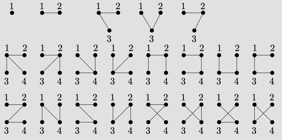
We can use padlock solitaire to give an elegant proof of Cayley’s famous theorem (actually first proved by Sylvester in 1857) that there are different trees on labeled vertices. The connection is given by observing that the distribution of keys into boxes can be represented by a directed graph on labeled vertices , where we put an edge directed from to if key is in box (so that opening box leads to opening box ).

Lemma 1: We win the game of solitaire if and only if is a tree rooted at vertex 1 with every edge directed away from the root.

Proof: We can eventually open box iff there is a path in from vertex 1 to vertex . If there is such a path to every vertex, then since there are only edges, must be a tree rooted at vertex 1 with every edge directed away from the root. Q.E.D.

Note that since any tree with a distinguished root can be uniquely oriented so that all edges are directed away from the root, Lemma 1 shows that the number of trees on is the same as the number of key distributions which result in winning the game of padlock solitaire.

Since there are different ways of distributing keys into boxes, Cayley’s formula is equivalent to the following assertion:

Lemma 2: The probability of winning padlock solitaire is .

Proof: We claim that the average number of hidden keys per unopened box, call it , is a martingale. Indeed, the unseen keys are equally likely to be in any of the remaining boxes, so that the expected change in when we open one of them is zero. More formally: at time , meaning after we have opened boxes, let be the the expected value of the number of hidden keys divided by the number of unopened boxes; then the sequence is a martingale. (Note that if we actually open the last box then becomes , so the stopping rule needed for this to work is that the solitaire game ends either when there are keys remaining but they’re all locked away, or as soon as we find the last key.)

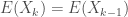
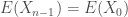
By the Optional Stopping Theorem, the expected value of when we begin is equal to the expected value of when we stop. At the beginning the value of is , and at the end it is probability of not winning (since if we find the last key and if we get stuck with all the remaining keys locked away). Therefore as claimed. Q.E.D.

This completes Wästlund’s derivation of Cayley’s formula. Here is (a sketch of) a self-contained version of his argument which does not require invoking the Optional Stopping Theorem. Let be the time at which we either find the last key or are unable to open any more boxes (but at least one unopened box remains). Define a sequence of random variables by setting for and for . The fact that the expected change in when we open one of the remaining boxes is zero, together with basic properties of expectation, implies that for all . We therefore have , i.e., , and thus .

Some other formulas that can be proved using martingales

Wästlund gives several other applications of “martingale enumeration” using padlock solitaire and its variations. For example, one can in this way enumerate (i) rooted forests, (ii) parking functions, (iii) spanning trees in uniform hypergraphs, (iv) trees with a prescribed degree sequence, (v) spanning trees in complete multi-partite graphs, and (vi) nilpotent matrices over finite fields. See Wästlund’s paper for details. We present here just one other application, to the famous formula for the Catalan numbers.

Recall that can be defined as the number of well-formed strings of length consisting of left-parentheses and right-parentheses, where a string is well-formed if, reading from left to right, we never see an excess of right-parentheses. The connection to padlock solitaire-type games is as follows. This time, instead of distributing the keys in advance, we shuffle a deck of red and black cards, letting the red cards correspond to the hidden keys in padlock solitaire (and to left-parentheses). We begin by opening box 1, and every time we open a box, we deal cards from the top of the deck until we get a black one. The red cards before that tell us which keys are in the box. One can show (see Section 10 of Wästlund’s paper) that (a) we lose the game if and only if at some point there is a black majority among the cards we have seen, and (b) the probability of winning the game is . Since the number of possible decks is , this gives the desired formula.

Concluding remarks

(1) A detailed online reference for stochastic processes, including martingales and the optional stopping theorem, is the website Random, especially Chapter 16. For a quick introduction to martingales and the Optional Stopping Theorem, see this blog post by Adam Lelkes, and for a proof see these notes by Scott LaLonde. See also this survey article by Joseph Doob himself.

(2) In this earlier post I discussed the Drunkard’s Walk; the solution to this problem can also be obtained using martingales. See, for example, this excellent expository article by J. Laurie Snell or Section 1.1.6 of this excellent book by Doyle and Snell. The Doyle-Snell book also explains, in an elementary way, the important connection between martingales and potential theory (harmonic functions, the Dirichlet problem, etc.).

(3) I previously wrote this blog post highlighting another ingenious proof by Johan Wästlund (on the solution to the famous Basel problem, solved by Euler). For another reason to join the Wästlund fan club, see http://wastlund.blogspot.com/2018/04/paradox-of-records.html

(4) There are numerous different proofs of Cayley’s formula in the literature, see for example Aigner and Ziegler’s Proofs from the Book and Tom Leinster’s exposition of Joyal’s proof. Another high-tech proof using ideas from probability theory – in this case branching processes – can be found here. My favorite proof first establishes a bijection between labeled trees on vertices and parking functions, and then counts parking functions using Pollak’s marvelous symmetry trick (see e.g. this survey paper by Catherine Yan).